Google Sheets has a very handy feature: tick boxes. The nice thing about a column of tick boxes is that you can see at a glance whether or not a task has been completed or a deadline met, or student work handed in, and so on.
To give you an idea of how the feature might be used, I’ve created a simple checklist of tasks that I, as a teacher, might need to complete in order to teach a group of students online. The checklist is:
Software installed?
Software tested?
Trial run organised?
Resources uploaded?
Online sessions scheduled?
Instructions to students sent out?
Calendar invitations sent out?
Here’s what it looks like in Google Sheets:
Tickbox 01 by Terry Freedman
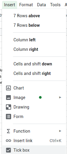
Notice that I’ve selected the cells under the heading “Done?”. That is so I can insert a tick box in each of them. You can do this by going to the Insert menu, and then clicking Tick box:
Tickbox 02 by Terry Freedman
Your spreadsheet will now look like this:
Tickbox 03 by Terry Freedman
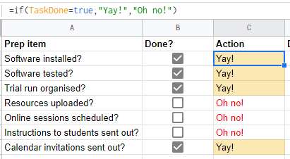
As you can see, I’ve inserted a formula in the first cell under “Action”, so let me explain this. The tick box is more than a pretty symbol: you can actually make use of it. If it is ticked, it has a property of True; if it is unticked, its property is False. That means you can insert an IF formula if you wish. In this case, the formula means:
If the box has been ticked, show the word “Yay!”; otherwise, show “Oh no!”.
Next, drag the formula down in order to copy it into each cell in that column, as far down as the end of the table:
Tickbox 04 by Terry Freedman
We can check whether it’s all working ok by ticking a few boxes:
Tickbox 05 by Terry Freedman
That is all looking good. Why not use some conditional formatting to highlight the cells in the Action column? You might think this is overkill, and in this example it definitely is because you can see the whole table at once. But imagine if the table was much bigger, it might be difficult to see the wood for the trees. A little colour could be useful.
To achieve this, I click on the column heading “C”, to select the whole column. Then click on Format->Conditional formatting:
Tickbox 06 by Terry Freedman
I enter the condition, which in this case is that the text in the cell is exactly equal to Yay!, and then select the formatting. I’ve decided to colour the cell in a cream colour.
Going through the same process, I have “told” the spreadsheet to make any text reading Oh no! in that column red. This is the result overall:
Tickbox 08 by Terry Freedman
This is all great so far, but can make he spreadsheet more helpful if I wish, by inserting a deadline for the task to be completed by. All I have to do is refine that IF statement a bit:
Tickbox 09 by Terry Freedman
This is what it means:
If the text in the Action column is “Oh no!”, set a new deadline of 7 days from today. Otherwise, just leave the cell blank (shown by opening and closing quotation marks with nothing between them).
But what if you want to change the number of days from today, or choose that number in the first place? In that case, all you have to do is designate a particular cell for the number of extra days to allow. I’ve used cell F1.
You can refine it even more by making that cell (F1 in my case) a named range. That is quite useful because it means that if you fall under a bus, anyone using the spreadsheet after your demise will be able to understand what is going on.
To name the cell, select it, right-click on it, and select Define the named range. Click on Add a range and then give it a name. In this case I’ve called it ExtraDays. I can now use this in my IF formula:
Tickbox 12 by Terry Freedman
As I’m sure you’ll agree, that makes the formula less obtuse. I could go much further in this direction by naming the cell range under Done as TaskDone (say), and the cell range under Action as Action. Now the formulas will appear like this:
TaskDone by Terry Freedman
Action, by Terry Freedman
Finally, if you wanted to, you could combine the date in the Deadline column with text. To do this I designated cell F2 as today’s date. The formula for that is simply =Today().
Here’s what the result looks like:
text and date, by Terry Freedman
Note that in order to combine the text “New deadline is” and the date, you have to do the following:
Use the =Text() function.
The syntax is =Text(cell ref, format).
Use & to link the text and the =Text function.
Include a space between the last word in your text and the closing quotation marks, otherwise there won’t be gap between the last word and the date.
Finally, note that in this case, because I’ve put today’s date in just one cell, I have to make that an absolute cell reference before copying it down. You do that by selecting the cell reference in the formula, and pressing F4. Then you can copy the formula down to all the relevant cells.
I hope you have found this brief tutorial useful. Do experiment to see what other uses you can find for the tick box.
If you found this article interesting and useful, why not subscribe to my newsletter, Digital Education? It’s been going since the year 2000, and has news, views and reviews for Computing and ed tech teachers.


